Regression is one of the main problems tackled by machine learning.
We define regression analysis as a set of statistical processes for estimating the relationship between a dependent variable (often called the target variable) and one or more independent variables (often called features). In Linear Regression we aim to find the best hyperplane that is able to predict the outcome variable starting from a set of features.
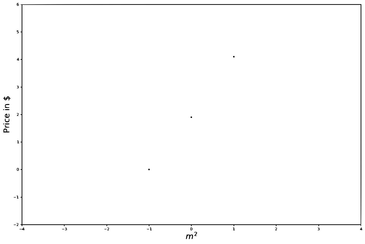
One trivial example could be estimating the price (target variable) of a house starting from the house’s dimension expressed in squared meters (\(m^2\)). In this case, since we are just considering one feature (the dimension of the house expressed in \(m^2\)) our hyperplane will consist of a simple line.
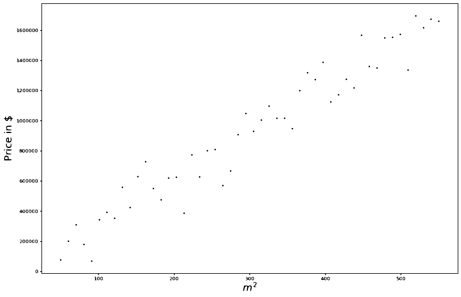
Each dot in the plot corresponds to a real data sample, namely a real correspondence among area and price. This is how our dataset would look like
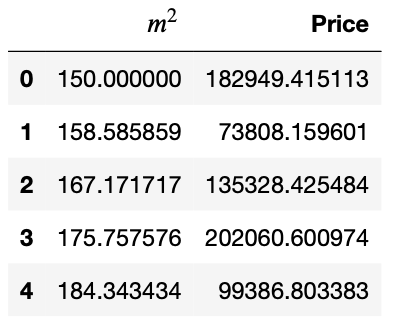
Our goal consists in finding the line that better explains the data we have been provided with.
This traduces in finding the best weights \(\textbf{w} = \begin{bmatrix}w_0 \\ w_1\end{bmatrix}\) such that \(w_0+w_1\cdot\left(\text{dimension in }m^2\right) \simeq\text{Price}\)
Now it’s time to introduce some formalism.
For the \(i_{th}\) data sample we call our target variable \(t_i\) , our features \(\mathbf{x}_i\) and the weights that we apply to our features \(\mathbf{w}\). Note that \(\mathbf{x}_i\) and \(\mathbf{w}\) are column vectors , while \(t_i\) is just a scalar.
Suppose we have \(n\) data samples and we consider \(m\) features, then we define:
The target vector
\[ \mathbf{t} = \begin{bmatrix}t_1\\ t_2\\ \vdots \\ t_n \end{bmatrix} \]
The dataset
\[ \mathbf{X}=\begin{bmatrix} \mathbf{x_1}^T \\ \mathbf{x_2}^T \\ \vdots \\ \mathbf{x}_n^T \end{bmatrix} = \begin{bmatrix} 1 && x_{11} && \cdots && x_{1m} \\ 1 && x_{21} && \cdots && x_{2m} \\ \vdots && \vdots && \ddots &&\vdots \\ 1 &&\cdots && \cdots &&x_{nm} \end{bmatrix} \]
Note that the \(1\) at the beginning of each row are just to take in account the bias \(w_0\) (that would be the intercept in our trivial example)
And the weights
\[ \mathbf{w}= \begin{bmatrix} w_0 \\ w_1 \\ w_2 \\ \vdots \\ w_m \end{bmatrix} \]
Then our prediction (that from now on we’ll call \(y\) ) for the \(i_{th}\) sample will be
\[ y_i = \mathbf{w}^T\mathbf{x}_i = \begin{bmatrix} w_0 && w_1 && w_2 && \cdots && w_m \end{bmatrix} \cdot \begin{bmatrix} 1 \\ x_{i1} \\ x_{i2} \\ \vdots \\ x_{im} \end{bmatrix} \]
And our prediction vector (which will have dimension \(n\times 1\)) will be computed as
\[ \mathbf{y}=\begin{bmatrix} 1 && x_{11} && \cdots && x_{1m} \\ 1 && x_{21} && \cdots && x_{2m} \\ \vdots && \vdots && \ddots &&\vdots \\ 1 &&\cdots && \cdots &&x_{nm} \end{bmatrix}\cdot\begin{bmatrix} w_0 \\ w_1 \\ \vdots \\ w_m \end{bmatrix}=\mathbf{X}\mathbf{w} \]
But how can we find the optimal weights? We do that by minimizing the so-called Mean Squared Error \(J(\mathbf{w})\).
\[ J(\mathbf{w}) =\\ \frac{1}{N}\left(\mathbf{t}-\mathbf{y}\right)^T\left(\mathbf{t}-\mathbf{y}\right)=\\\frac{1}{N}\left(\mathbf{t}-\mathbf{X}\mathbf{w}\right)^T\left(\mathbf{t}-\mathbf{X}\mathbf{w}\right) \]
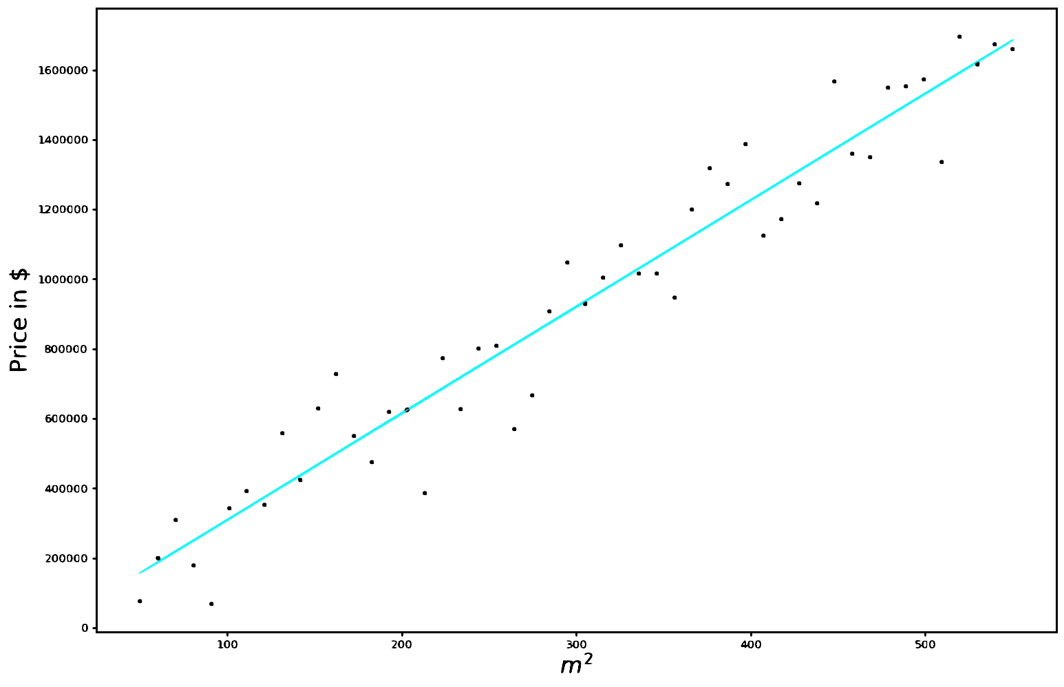
Where \(\epsilon_i\) is just the difference between the target values \(t_i\) and our predictions \(y_i\),
\[ \begin{bmatrix} t_1-y_1 \\ t_2-y_2 \\ t_3-y_3 \\ \vdots \\ t_n-y_n \end{bmatrix} = \begin{bmatrix} \epsilon_1 \\ \epsilon_2 \\ \epsilon_3 \\ \vdots \\ \epsilon_n \end{bmatrix} \]
To have a visual understanding of what we’re talking about, the various \(\epsilon_i\) corresponds to the green segments in the image below.
Our cost function is just the Mean Squared Error
\[ J(\mathbf{w}) = \frac{1}{N}\sum_{i=1}^n\epsilon_i^2 \]
Since we would like to minimize this quantity, we derive with respect to \(\mathbf{w}\) and set the derivative equal to \(0\) .
\[ J\left(\mathbf{w}\right) = \frac{1}{N}\left(\mathbf{t}-\mathbf{X}\mathbf{w}\right)^T\left(\mathbf{t}-\mathbf{X}\mathbf{w}\right)\\\frac{\partial J(\mathbf{w})}{\partial \mathbf{w}} = -\frac{2}{N}\mathbf{X}^T\left(\mathbf{t}-\mathbf{X}\mathbf{w}\right) =0 \]
Which is equivalent to
\[ \mathbf{X}^T\left(\mathbf{t}-\mathbf{X}\mathbf{w}\right)=0 \]
We then isolate the weights
\[ \mathbf{X}^T\mathbf{t}=\mathbf{X}^T\mathbf{X}\mathbf{w}\\ \mathbf{w}=\left(\mathbf{X}^T\mathbf{X}\right)^{-1}\mathbf{X}^T\mathbf{t} \]
And that’s all!
Now, before tackling the problems relative with such closed form solution, it is useful to introduce the parameters-space, i.e. the space representing all the possible solutions \((w)\) of our problem: in our trivial example this space corresponds to all the possible points \(w:(w_0,w_1) \in \mathbb{R}^2\), each of this points traduces in a different predictor (line) in the features-space as you can see in the animation below.
Let’s talk now about some problems that can arise from the closed form solution
- The inverse of \(\left(\mathbf{X}^T\mathbf{X}\right)\) is computationally expensive when the number of features is high, being the temporal complexity of such inversion \(\mathcal{O}(m^3)\) (Note that \(\left(\mathbf{X}^T\mathbf{X}\right)\) has dimensionality equal to \((m+1)\times (m+1)\) )
- The matrix \(\left(\mathbf{X}^T\mathbf{X}\right)\) isn’t always invertible since \(\mathbf{X}^T\mathbf{X}\) could contain linearly dependent rows, which implies a null determinant. In such case we’d have infinite solutions for \(\mathbf{w}\).
In order to show this last drawback we’ll use a toy example:
We have to find a valid predictor for a dataset which contains just three samples.
We solve by means of the closed form solution:
\[ \mathbf{X}\mathbf{w}=\mathbf{t} \]
\[ \begin{bmatrix}1 && 1\\1 && 0\\1 && -1\\\end{bmatrix}\cdot\begin{bmatrix}\mathbf{w}_0\\\mathbf{w}_1\\\end{bmatrix}=\begin{bmatrix}4.1\\1.9\\0\end{bmatrix} \]
\[ \mathbf{w}=\left(\mathbf{X}^T\mathbf{X}\right)^{-1}\mathbf{X}^T\mathbf{t} \]
\[ \mathbf{w} = \begin{bmatrix} \begin{bmatrix} 1 && 1 && 1\\ 1 && 0 && -1\\ \end{bmatrix} \cdot \begin{bmatrix} 1 && 1\\ 1 && 0\\ 1 && -1\\ \end{bmatrix} \end{bmatrix} ^{-1} \cdot \begin{bmatrix} 1 && 1 && 1\\ 1 && 0 && -1\\ \end{bmatrix} \begin{bmatrix} 4.1\\ 1.9\\ 0 \end{bmatrix} \]
\[ \mathbf{w} = \begin{bmatrix} 3 && 0\\ 0 && 2 \end{bmatrix} ^{-1} \cdot \begin{bmatrix} 1 && 1 && 1\\ 1 && 0 && -1\\ \end{bmatrix} \cdot \begin{bmatrix} 4.1\\ 1.9\\ 0 \end{bmatrix} \]
\[ \mathbf{w} = \frac{1}{6} \begin{bmatrix} 2 && 0\\ 0 && 3 \end{bmatrix} \cdot \begin{bmatrix} 1 && 1 && 1\\ 1 && 0 && -1\\ \end{bmatrix} \cdot \begin{bmatrix} 4.1\\ 1.9\\ 0 \end{bmatrix} \]
\[ \mathbf{w} = \begin{bmatrix} \frac{1}{3} && 0\\ 0 && \frac{1}{2} \\ \end{bmatrix} \cdot \begin{bmatrix} 1 && 1 && 1\\ 1 && 0 && -1\\ \end{bmatrix} \cdot \begin{bmatrix} 4.1\\ 1.9\\ 0 \end{bmatrix} \]
\[ \mathbf{w} = \begin{bmatrix} \frac{1}{3} && \frac{1}{3} && \frac{1}{3}\\ \frac{1}{2} && 0 && -\frac{1}{2} \end{bmatrix} \cdot \begin{bmatrix} 4.1\\ 1.9\\ 0 \end{bmatrix} \]
\[ \mathbf{w} = \begin{bmatrix} 2.00\\ 2.05 \end{bmatrix} \]
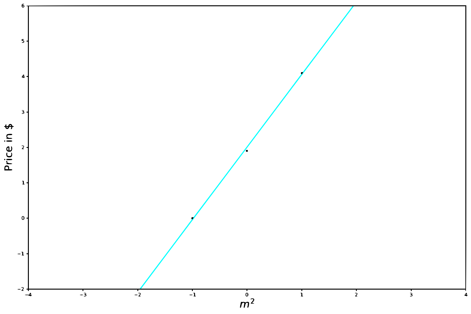
In this case \(\mathbf{X}^T\mathbf{X}\) is invertible and, if we plot the cost function \(J(\mathbf{w})\) in the parameter space, we can see that \(J(\mathbf{w})\) is a convex function with one single minimum and a well defined bowl shape. This minimum corresponds to the point \(\mathbf{w} = \begin{bmatrix} 2.00\\ 2.05 \end{bmatrix}\), i.e. the blue dot which appears at the base of the bowl.
Which corresponds to the following predictor line:
The above example is the ideal scenario, but it is not always the one you’ll be dealing with. In fact there are some observations to be done regarding the dataset to be used:
Now let’s compute the closed form solution for another example:
\[ \begin{bmatrix}m^2 && price\\2 && 2\\2 && 4\\2 && 6\\\end{bmatrix} \]
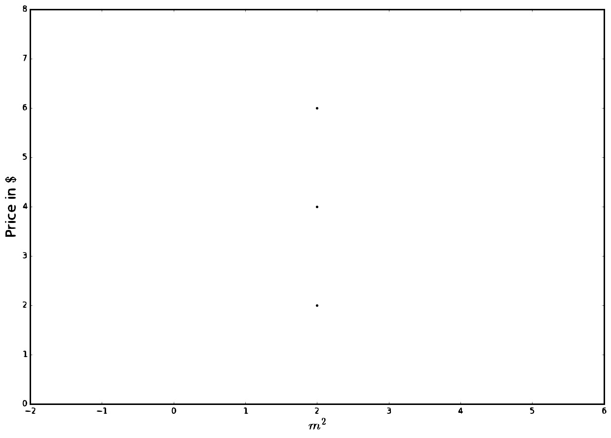
Here our data samples are pretty bad since there doesn’t seem to be any correlation between the independent variable \((m^2)\) and the dependent variable \((price)\). We will observe that the inversion of the matrix \(\mathbf{X}^T\mathbf{X}\) becomes problematic.
\[ \mathbf{X}\mathbf{w}=\mathbf{t} \]
\[ \begin{bmatrix}1 && 2\\1 && 2\\1 && 2\\\end{bmatrix}\cdot\begin{bmatrix}\mathbf{w}_0\\\mathbf{w}_1\\\end{bmatrix}=\begin{bmatrix}2\\4\\6\end{bmatrix} \]
\[ \mathbf{w}=\left(\mathbf{X}^T\mathbf{X}\right)^{-1}\mathbf{X}^T\mathbf{t} \]
\[ \mathbf{w} =\begin{bmatrix}\begin{bmatrix}1 && 1 && 1\\2 && 2 && 2\\\end{bmatrix}\cdot\begin{bmatrix}1 && 2\\1 && 2\\1 && 2\\\end{bmatrix}\end{bmatrix}^{-1}\cdot\begin{bmatrix}1 && 1 && 1\\2 && 2 && 2\\\end{bmatrix}\begin{bmatrix}2\\4\\6\end{bmatrix} \]
\[ \mathbf{w} = \begin{bmatrix} 3&& 6\\6 && 12\end{bmatrix}^{-1}\cdot\begin{bmatrix}1 && 1 && 1\\2 && 2 && 2\\\end{bmatrix}\cdot\begin{bmatrix}2\\4\\6\end{bmatrix} \]
As you can see here we can’t invert \[ \begin{bmatrix} 3 && 6 \\ 6 && 12 \end{bmatrix} \] since its determinant would be \(0\) !
By plotting the cost function \(J(\mathbf{w})\) we would obtain a sort of parabolic cylinder
whose minimum has infinite solutions (that we can find by gradient-based techniques).
Lastly it is opportune to remember that our dataset needs to have a number of samples greater than the number of parameters to be learnt. Being \(m\) the number of features of each sample and \(n\) the number of samples in our dataset, we need to satisfy the constraint \(n>m+1\). Let’s reason why through a simple example. Suppose that you have been asked to find the model that best explains a dataset made of \(2\) samples \((n=2)\). Suppose that each sample is represented by \(2\) features \((m=2)\) and that we need to predict a value \(t\). In this scenario we are not satisfying the constraint since \(2\not>2+1\). What are the consequences? Of course we will get a perfect fit! There are infinite planes \((w_0+w_1x_1+w_2x_2=0)\) which pass through two points!
We’ll find at least a model that passes through all the data, more specifically we’d find one solution in the \(n=m+1\) case, and infinite solutions in the \(n<m+1\) case. We have found a very bad family of models because they are an exact representation of the training data, which translates into a very obvious overfitting problem. Generally we want \(n >> m\).