Let’s start with a question: what is Generative Modeling?
Generative modeling is an unsupervised learning task in machine learning that involves automatically discovering and learning the regularities or patterns in input data in such a way that the model can be used to generate or output new examples that plausibly could have been drawn from the original dataset.
GANs are a clever way of training a generative model by framing the problem as a supervised learning problem with two sub-models: the generator model that we train to generate new examples, and the discriminator model that tries to classify examples as either real (from the domain) or fake (generated).
Formulation
Generator \(\mathcal{G}\): produces realistic samples e.g. taking as input some random noise. \(\mathcal{G}\) tries to fool the discriminator
Discriminator \(\mathcal{D}\) that takes as input an image and assess whether it is real or generated by \(\mathcal{G}\)
Both \(\mathcal{D}\) and \(\mathcal{G}\) are conveniently chosen as MLPs. The generative process depends on two networks:
\(\mathcal{D} =\mathcal{D}(\mathbf{x},\theta_d)\)
\(\mathcal{G} =\mathcal{G}(\mathbf{z},\theta_g)\)
\(\theta_g\) and \(\theta_d\) are the network parameters, \(\mathbf{x}\in\mathbb{R}^n\) is an input image (either real or generated by \(\mathcal{G}\)) and \(\mathbf{z}\in\mathbb{R}^d\) is some random noise to be fed to the generator. We suppose that \(\mathbf{x}\) is sampled from a distribution \(p_{data}\) \((\)i.e. \(\mathbf{x}\sim p_{data}(\mathbf{x}))\) and \(\mathbf{z}\) is sampled from a distribution \(p_z\) \((\)i.e. \(\mathbf{z}\sim p_z(\mathbf{z}))\). Our Discriminator’s output is to be seen as the probability that the input image comes from the data and not from the generator: \[ \mathcal{D}(\cdot,\theta_d):\mathbb{R}^n \to [0,1] \]
The generator gives as output a generated image: \[ \mathcal{G}(\cdot,\theta_d):\mathbb{R}^d \to \mathbb{R}^n \] A good discriminator is such that:
\(\mathcal{D}(\mathbf{x},\theta_d)\) is maximum when \(\mathbf{x} \in X\) (i.e. \(\mathbf{x}\) is sampled for the real images dataset \(X\))
\(1 - \mathcal{D}(\mathbf{x},\theta_d)\) is maximum when \(\mathbf{x}\) was generated by \(\mathcal{G}\)
\(1 - \mathcal{D}(\mathcal{G}(\mathbf{z},\theta_g),\theta_d)\) is maximum when \(\mathbf{z} \sim p_z(\mathbb{z})\)
Training \(\mathcal{D}\) consists in maximizing the binary cross-entropy:
\[ \underset{\theta_d}{\text{max}} \left(\ \mathbb{E}_{\mathbf{x}\sim p_{data}(\mathbf{x})} [\log\mathcal{D}(\mathbf{x},\theta_d)] + \mathbb{E}_{\mathbf{z}\sim p_z(\mathbf{z})} \log[1-\mathcal{D}(\mathcal{G}(\mathbf{z},\theta_g),\theta_d)] \ \right) \]
Where
- \(\mathcal{D}(\mathbf{x},\theta_d)\) has to be \(1\) since \(\mathbf{x} \sim p_{data}(\mathbf{x})\), namely images are real.
- \(\mathcal{D}(\mathcal{G}(\mathbf{z},\theta_g),\theta_d)\) has to be \(0\) since \(\mathcal{G}(\mathbf{z},\theta_g)\) is a generated (fake) image.
A good generator \(\mathcal{G}\) is one that makes \(\mathcal{D}\) fail:
\[ \underset{\theta_g}{\text{min}} \left( \underset{\theta_d}{\text{max}} \left(\ \mathbb{E}_{\mathbf{x}\sim p_{data}(\mathbf{x})} [\log\mathcal{D}(\mathbf{x},\theta_d)] + \mathbb{E}_{\mathbf{z}\sim p_z(\mathbf{z})} \log[1-\mathcal{D}(\mathcal{G}(\mathbf{z},\theta_g),\theta_d)] \ \right) \right) \]
Optimizing \(\mathcal{D}\) to completion in the inner loop of training is computationally prohibitive, and on finite datasets would result in overfitting. Instead, we alternate between \(k\) steps of optimizing \(\mathcal{D}\) and one step of optimizing \(\mathcal{G}\). This results in \(\mathcal{D}\) being maintained near its optimal solution, as long as \(\mathcal{G}\) changes slowly enough.
Let’s schematize it:
We need to solve by an iterative numerical approach the min max game shown at \((4)\). In order to do so we alternate:
\(k\)-steps of Stochastic Gradient Ascent w.r.t. \(\theta_d\) to solve
\[ \underset{\theta_d}{\text{max}} \left(\ \mathbb{E}_{\mathbf{x}\sim p_{data}(\mathbf{x})} [\log\mathcal{D}(\mathbf{x},\theta_d)] + \mathbb{E}_{\mathbf{z}\sim p_z(\mathbf{z})} \log[1-\mathcal{D}(\mathcal{G}(\mathbf{z},\theta_g),\theta_d)] \ \right) \]
\(1\)-step of Stochastic Gradient Descent w.r.t. \(\theta_g\) being \(\theta_d\) fixed:
\[ \underset{\theta_g}{\text{min}} \left(\ \mathbb{E}_{\mathbf{x}\sim p_{data}(\mathbf{x})} [\log\mathcal{D}(\mathbf{x},\theta_d)] + \mathbb{E}_{\mathbf{z}\sim p_z(\mathbf{z})} \log[1-\mathcal{D}(\mathcal{G}(\mathbf{z},\theta_g),\theta_d)] \ \right) \]
i.e. (the removed term does not depend on \(\theta_g\))
\[ \underset{\theta_g}{\text{min}} \left(\ \mathbb{E}_{\mathbf{z}\sim p_z(\mathbf{z})} [\log(1-\mathcal{D}(\mathcal{G}(\mathbf{z},\theta_g),\theta_d))] \ \right) \]
i.e.
\[ \underset{\theta_g}{\text{max}} \left(\ \mathbb{E}_{\mathbf{z}\sim\phi_z} [\log\mathcal{D}(\mathcal{G}(\mathbf{z},\theta_g),\theta_d)] \ \right) \]
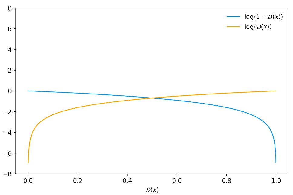
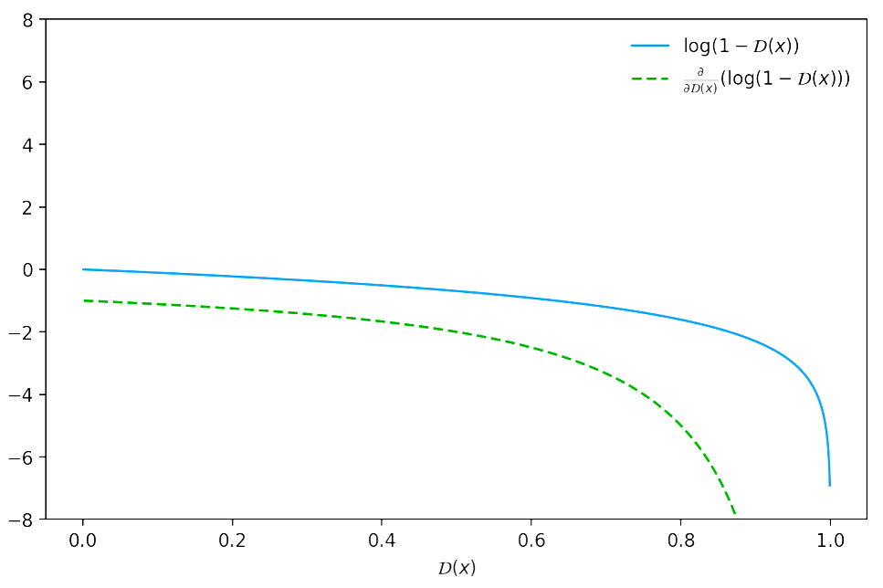
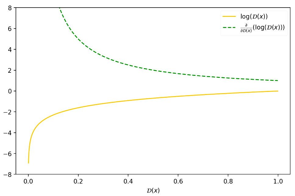
There is a reason why Goodfellow proposed to optimize \(\log(\mathcal{D}(\cdot))\) instead of \(\log(1-\mathcal{D}(\cdot))\). If we try to descend the gradient of \(\log(1-\mathcal{D}(x))\), we notice that at the beginning of the training process, when the generated samples would be easily classified as “fake” (i.e. \(\mathcal{D}(x) \sim 0\)), there would be too few gradient in order to learn properly!
We have the following value function for our min-max problem:
\[ V(\mathcal{G},\mathcal{D}) = \mathbb{E}_{\mathbf{x}\sim p_{\text{data}}(\mathbf{x})}\log(\mathcal{D}(\mathbf{x}))\mathbf{x}+\mathbb{E}_{\mathbf{z}\sim p_{z}(\mathbf{z})}\log(1-\mathcal{D}(\mathcal{G}(\mathbf{z}))d\mathbf{z} \]
\[ =\int_{\mathbf{x}}p_{\text{data}}(\mathbf{x})\log(\mathcal{D}(\mathbf{x}))d\mathbf{x} + \int_{\mathbf{z}}p_{\mathbf{z}}(\mathbf{z})\log(1-\mathcal{D}(\mathcal{G}(\mathbf{z}))d\mathbf{z} \]
\[ =\int_{\mathbf{x}} \left( p_{\text{data}}(\mathbf{x}) \log(\mathcal{D}(\mathbf{x})) + p_{g}(\mathbf{x}) \log(1-\mathcal{D}(\mathbf{x})) \right) d\mathbf{x} \]
This last equality comes from the Radon-Nikodym Theorem of measure theory and it’s sometimes referred as the Law Of The Unconscious Statistician (or LOTUS Theorem) since students have been accused of using the identity without realizing that it must be treated as the result of a rigorously proved theorem, not merely a definition (if you want the full proof check this out! )
\[ V(\mathcal{G},\mathcal{D}) =\int_{\mathbf{x}} \left( p_{\text{data}}(\mathbf{x}) \log(\mathcal{D}(\mathbf{x})) + p_{g}(\mathbf{x}) \log(1-\mathcal{D}(\mathbf{x})) \right) d\mathbf{x} \]
Let’s first consider the optimal discriminator \(\mathcal{D}\) for any given generator \(\mathcal{G}\). The training criterion for the discriminator \(\mathcal{D}\), given any generator \(\mathcal{G}\), is to maximize the quantity defined below:
\[ \underset{\mathcal{D}}{\text{argmax}}\left(V(\mathcal{G},\mathcal{D})\right) =\underset{\mathcal{D}}{\text{argmax}}\left(\int_{\mathbf{x}} \left( p_{\text{data}}(\mathbf{x}) \log(\mathcal{D}(\mathbf{x})) + p_{g}(\mathbf{x}) \log(1-\mathcal{D}(\mathbf{x})) \right) d\mathbf{x} \right) \]
For the individual sample \(\mathbf{x}\) we derive \(V(\mathcal{G},\mathcal{D})\) w.r.t. \(\mathcal{D}(\mathbf{x})\) and we equal this quantity to \(0\) in order to find the optimal discriminator \(\mathcal{D}(\mathbf{x})^{*}\)
\[ \frac{d}{d\mathcal{D}(\mathbf{x})}\left( p_{\text{data}}(\mathbf{x}) \log(\mathcal{D}(\mathbf{x})) + p_{g}(\mathbf{x}) \log(1-\mathcal{D}(\mathbf{x})) \right) =0 \]
\[ \frac{p_{data}(\mathbf{x})}{\mathcal{D}^{*}(\mathbf{x})} - \frac{p_{g}(\mathbf{x})}{1-\mathcal{D}^{*}(\mathbf{x})}=0 \]
\[ \frac{p_{data}(\mathbf{x})(1-\mathcal{D}^{*}(\mathbf{x}))-p_{g}(\mathbf{x})\mathcal{D}^{*}(\mathbf{x})}{\mathcal{D}^{*}(\mathbf{x})(1-\mathcal{D}^{*}(\mathbf{x}))} =0 \]
\[ \frac{p_{data}(\mathbf{x})-p_{data}(\mathbf{x})\mathcal{D}^{*}(\mathbf{x})-p_{g}(\mathbf{x})\mathcal{D}^{*}(\mathbf{x})}{\mathcal{D}^{*}(\mathbf{x})(1-\mathcal{D}^{*}(\mathbf{x}))} = 0 \]
\[ p_{data}(\mathbf{x})-p_{data}(\mathbf{x})\mathcal{D}^{*}(\mathbf{x})-p_{g}(\mathbf{x})\mathcal{D}^{*}(\mathbf{x}) = 0 \]
\[ p_{data}(\mathbf{x})-\mathcal{D}^{*}(\mathbf{x})\left(p_{data}(\mathbf{x})+p_{g}(\mathbf{x})\right) = 0 \]
\[ \color{blue}{\mathcal{D}^{*}(\mathbf{x}) = \frac{p_{data}(\mathbf{x})}{p_{data}(\mathbf{x})+p_{g}(\mathbf{x})} } \]
Does this point represent a maximum? we have to check if the second derivative calculated in \(\mathcal{D}^{\star}\) is negative.
\[ \frac{d}{d\mathcal{D}(\mathbf{x})}\left( p_{\text{data}}(\mathbf{x}) \log(\mathcal{D}(\mathbf{x})) + p_{g}(\mathbf{x}) \log(1-\mathcal{D}(\mathbf{x})) \right) = \frac{p_{data}(\mathbf{x})}{\mathcal{D}(\mathbf{x})} - \frac{p_{g}(\mathbf{x})}{1-\mathcal{D}(\mathbf{x})} \]
\[ \frac{d^2}{d^2\mathcal{D}(\mathbf{x})}\left( p_{\text{data}}(\mathbf{x}) \log(\mathcal{D}(\mathbf{x})) + p_{g}(\mathbf{x}) \log(1-\mathcal{D}(\mathbf{x})) \right) = \frac{d}{d\mathcal{D}(\mathbf{x})}\left(\frac{p_{data}(\mathbf{x})}{\mathcal{D}(\mathbf{x})} - \frac{p_{g}(\mathbf{x})}{1-\mathcal{D}(\mathbf{x})}\right) \]
\[ \frac{d}{d\mathcal{D}(\mathbf{x})}\left(\frac{p_{data}(\mathbf{x})}{\mathcal{D}(\mathbf{x})} - \frac{p_{g}(\mathbf{x})}{1-\mathcal{D}(\mathbf{x})}\right) = -\frac{p_{data}(\mathbf{x})}{\mathcal{D}^2(\mathbf{x})} - \frac{p_{g}(\mathbf{x})}{\left(1-\mathcal{D}(\mathbf{x})\right)^2} < 0 \]
The quantity above is negative for every \(\mathcal{D}\), \(\mathcal{D}^*\) included, since \(p_{data}(\mathbf{x})\) and \(p_g(\mathbf{x})\) are between \(0\) and \(1\).
We then can plug \(\mathcal{D^{\star}}\) into \(\mathcal{V(G,D)}\) and find the optimal generator \(\mathcal{G^{\star}}\) as:
\[ \int_{\mathbf{x}}\left(p_{\text{data}}(\mathbf{x}) \log(\mathcal{D}^{\star}(\mathbf{x})) + p_{g}(\mathbf{x}) \log(1-\mathcal{D}^{\star}(\mathbf{x}))\right)d\mathbf{x} \]
\[ \mathcal{G}^{\star} =\underset{\mathcal{G}}{\text{argmin}}\left(\int_{\mathbf{x}} \left( p_{\text{data}}(\mathbf{x}) \log\left(\frac{p_{data}(\mathbf{x})}{p_{data}(\mathbf{x})+p_{g}(\mathbf{x})}\right) + p_{g}(\mathbf{x}) \log\left(1-\frac{p_{data}(\mathbf{x})}{p_{data}(\mathbf{x})+p_{g}(\mathbf{x})}\right) \right) d\mathbf{x} \right) \]
\[ \mathcal{G}^{\star} =\underset{\mathcal{G}}{\text{argmin}}\left(\int_{\mathbf{x}} \left( p_{\text{data}}(\mathbf{x}) \log\left(\frac{p_{data}(\mathbf{x})}{p_{data}(\mathbf{x})+p_{g}(\mathbf{x})}\right) + p_{g}(\mathbf{x}) \log\left(\frac{p_{g}(\mathbf{x})}{p_{data}(\mathbf{x})+p_{g}(\mathbf{x})}\right) \right) d\mathbf{x} \right) \]
\[ \mathcal{G}^{\star}=\underset{\mathcal{G}}{\text{argmin}}\left( \int_{\mathbf{x}} \left( p_{\text{data}}(\mathbf{x}) \left(\log 2 - \log 2\right) + p_{\text{data}}(\mathbf{x}) \log\left(\frac{p_{data}(\mathbf{x})}{p_{data}(\mathbf{x})+p_{g}(\mathbf{x})}\right) \\ + p_{\text{g}}(\mathbf{x}) \left(\log 2 - \log 2\right) + p_{g}(\mathbf{x}) \log\left(\frac{p_{g}(\mathbf{x})}{p_{data}(\mathbf{x})+p_{g}(\mathbf{x})}\right) \right) d\mathbf{x} \right) \]
\[ \mathcal{G}^{\star}=\underset{\mathcal{G}}{\text{argmin}}\left( -\log 2\int_{\mathbf{x}}\left(p_g(\mathbf{x})+p_{data}(\mathbf{x})\right)d\mathbf{x} + \int_{\mathbf{x}} p_{\text{data}}(\mathbf{x}) \left(\log 2 + \log\left(\frac{p_{data}(\mathbf{x})}{p_{data}(\mathbf{x})+p_{g}(\mathbf{x})} \right)\right)d\mathbf{x}\\ + \int_{\mathbf{x}} p_{\text{g}}(\mathbf{x}) \left(\log 2 + \log\left(\frac{p_{g}(\mathbf{x})}{p_{data}(\mathbf{x})+p_{g}(\mathbf{x})}\right)\right)d\mathbf{x} \right) \]
\[ \mathcal{G}^{\star}=\underset{\mathcal{G}}{\text{argmin}}\left( -\log 2 \cdot (2) + \int_{\mathbf{x}} p_{\text{data}}(\mathbf{x}) \log\left(2\cdot\frac{p_{data}(\mathbf{x})}{p_{data}(\mathbf{x})+p_{g}(\mathbf{x})} \right)d\mathbf{x}\\ + \int_{\mathbf{x}} p_{\text{g}}(\mathbf{x}) \log\left(2\cdot\frac{p_{g}(\mathbf{x})}{p_{data}(\mathbf{x})+p_{g}(\mathbf{x})}\right)d\mathbf{x} \right) \]
\[ \mathcal{G}^{\star}=\underset{\mathcal{G}}{\text{argmin}}\left( -\log 2^2 + \int_{\mathbf{x}} p_{\text{data}}(\mathbf{x}) \log\left(\frac{p_{data}(\mathbf{x})}{\frac{p_{data}(\mathbf{x})+p_{g}(\mathbf{x})}{2}} \right)d\mathbf{x}\\ + \int_{\mathbf{x}} p_{\text{g}}(\mathbf{x}) \log\left(\frac{p_{g}(\mathbf{x})}{\frac{p_{data}(\mathbf{x})+p_{g}(\mathbf{x})}{2}}\right)d\mathbf{x} \right) \]
\[ \mathcal{G}^{\star}=\underset{\mathcal{G}}{\text{argmin}}\left( -\log 4 + \mathit{KL}\left(p_{data}||\frac{p_g+p_{data}}{2}\right) + \mathit{KL}\left(p_{g}||\frac{p_g+p_{data}}{2}\right) \right) \]
\[ \color{blue}{\mathcal{G}^{\star}=\underset{\mathcal{G}}{\text{argmin}}\left( -\log 4 + 2\cdot\mathit{JSD}(p_{data}||p_g)\right)} \]
Where the Kullback-Leibler divergence (KL) and the Jenson-Shannon divergence (JSD) are quantities that measure the difference between two distributions and we know that \(\mathit{JSD}(p_{data}\vert\vert p_g)=0\) only when \(p_{data} = p_g\) !
\[ \implies V(\mathcal{D}^{\star}_{\mathcal{G}},\mathcal{G}) = -\log 4 \]
Theorem \(1\):
The global minimum of the virtual training criterion \[V(\mathcal{D}^{\star}_{\mathcal{G}},\mathcal{G})\] is achieved if and only if \(p_{g}=p_{data}\). At that point, \(V(\mathcal{D}^{\star}_{\mathcal{G}},\mathcal{G})\) achieves the value \(−\log 4\).
Besides, that was what we expected! We wanted our generator to learn the same distribution which generated the data. If we know that \(p_{data} = p_g\) then it’s trivial to observe that at the end of the training process the optimal discriminator will be forced to output \(0.5\) since it won’t be able to distinguish between real and fake samples anymore.
\[ \color{blue}{\mathcal{D}^{\star}(\mathbf{x}) = \frac{p_{data}(\mathbf{x})}{p_{data}(\mathbf{x})+p_{g}(\mathbf{x})} = \frac{1}{2}} \]
But does this converge?
Well, as stated in the original Paper:
If \(\mathcal{G}\) and \(\mathcal{D}\) have enough capacity, and at each step of our algorithm, the discriminator is allowed to reach its optimum given \(\mathcal{G}\) and \(p_g\) is updated so as to improve the criterion \[ \mathbb{E}_{\mathbf{x}\sim p_{data}}\left[\log\mathcal{D}^{\star}_{G}(\mathbf{x})\right] + \mathbb{E}_{\mathbf{x}\sim p_{g}}\left[\log(1-\mathcal{D}^{\star}_{G}(\mathbf{x}))\right] \]
then \(p_g\) converges to \(p_{data}\).
Proof:
Consider \(V(\mathcal{G,D})= U(p_g,\mathcal{D})\) as a function of \(p_g\) as done in the above criterion. Note that \(U(p_g,\mathcal{D})\) is convex in \(p_g\).
The subderivatives of a supremum of convex functions include the derivative of the function at the point where the maximum is attained. In other words, if \(f(x)=\sup_{\alpha\in\mathcal{A}}f_\alpha(x)\) and \(f_\alpha(x)\) is convex in \(x\) for every \(\alpha\) , then \(\partial f_\beta(x) \in \partial f\) if \(\beta=\arg\sup_{\alpha\in\mathcal{A}}f_\alpha(x)\). This is equivalent to computing a gradient descent update for \(p_g\) at the optimal \(\mathcal{D}\) given the corresponding \(\mathcal{G}\). \(\sup_\mathcal{D}U(p_g,\mathcal{D})\) is convex in \(p_g\) with a unique global optima as proven in Theorem \(1\), therefore with sufficiently small updates of \(p_g\), \(p_g\) converges to \(p_x\), concluding the proof.
In practice, adversarial nets represent a limited family of \(p_g\) distributions via the function \(\mathcal{G}(\mathbf{z};\theta_g)\), and we optimise \(\theta_g\) rather than \(p_g\) itself. Using a multilayer perceptron to define \(\mathcal{G}\) introduces multiple critical points in parameter space. However, the excellent performance of multilayer perceptrons in practice suggests that they are a reasonable model to use despite their lack of theoretical guarantees.